Day: 22 Jul 2019

In the past few days I’ve been following the playback of the Apollo 11 mission in “real time” (delayed exactly 50 years) at https://apolloinrealtime.org/11/.  Among all the news related to the 50th anniversary of the Apollo 11 moon landing I also found an article from NPR about about 3 different approaches to how to get to the moon, and how the one they used almost wasn’t ( Meet John Houbolt: He Figured Out How To Go To The Moon, But Few Were Listening).  This has caused me to think a bit about how to visualize the gravitational potential between the Moon and Earth (“cislunar”¹) and how the path chosen for the mission was somewhat like a car driving up a mountain to go over a pass to a valley on the other side.   As a result, I wrote a short Python script to show the potential as a surface over a 2 dimensional plane, and then “played” with the color map and other effects to highlight that “mountain pass” between the Earth and the Moon.

I’ve included a derivation of the equation for the gravitational potential for those who are interested, but it’s down at the end (for those who are not).  The Python script which was used to create all these images is at http://www.spy-hill.net/myers/astro/cislunar/CisLunar.py.  See the comments in the code for the small changes needed to turn one into the other.

Visualized as a Terrain Map

This first plot shows the potential surface with a color map commonly used for terrain, where sea level is blue, lowlands are green, mountains are brown, and mountain tops are white:

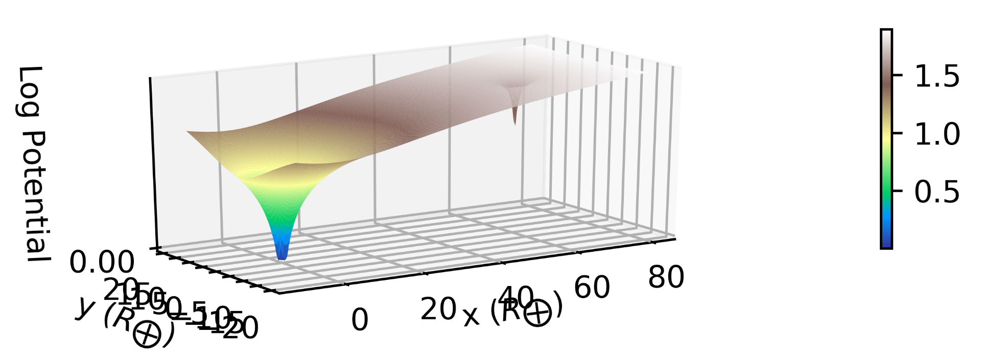
The idea is that going to the Moon is like climbing a mountain. Going up a hill increases your gravitational potential energy, and the same is true when a spacecraft goes up this surface on the way to the moon.  The blue at the bottom of the left potential well is the Earth, and the dimple up the hill to the right is the Moon.

The x and y coordinates on this figure are measured in units of the radius of the Earth (symbol R_⊕). The vertical scale is logarithmic² to make it easier to see the variation on a reasonable scale. The horizontal spacing is to scale: the Moon is a little over 60 Earth radii from the Earth.   The bottom of each potential well is flat and to scale.  That shows the small size of the Earth and the Moon compared to the distance between them.

Viewing from the side shows the variation in “elevation” a little better:

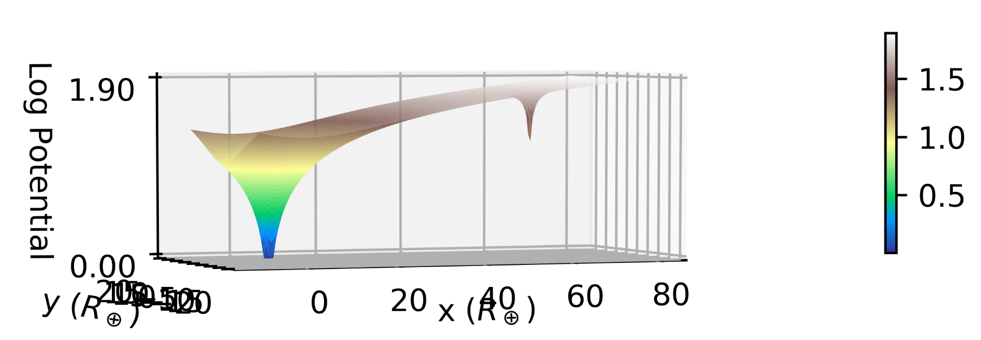
Now you can at least start seeing the idea that going to the moon is like going up a mountain and then down into a valley.

Visualized with Color Contours

The problem with the images above is that the color map changes gradually, so you cannot see the subtle changes at the “mountain pass”.   To help visualize that more clearly I switched to an artificial color map³ which varies between colors more often and uses more distinct colors.  Here is the result:

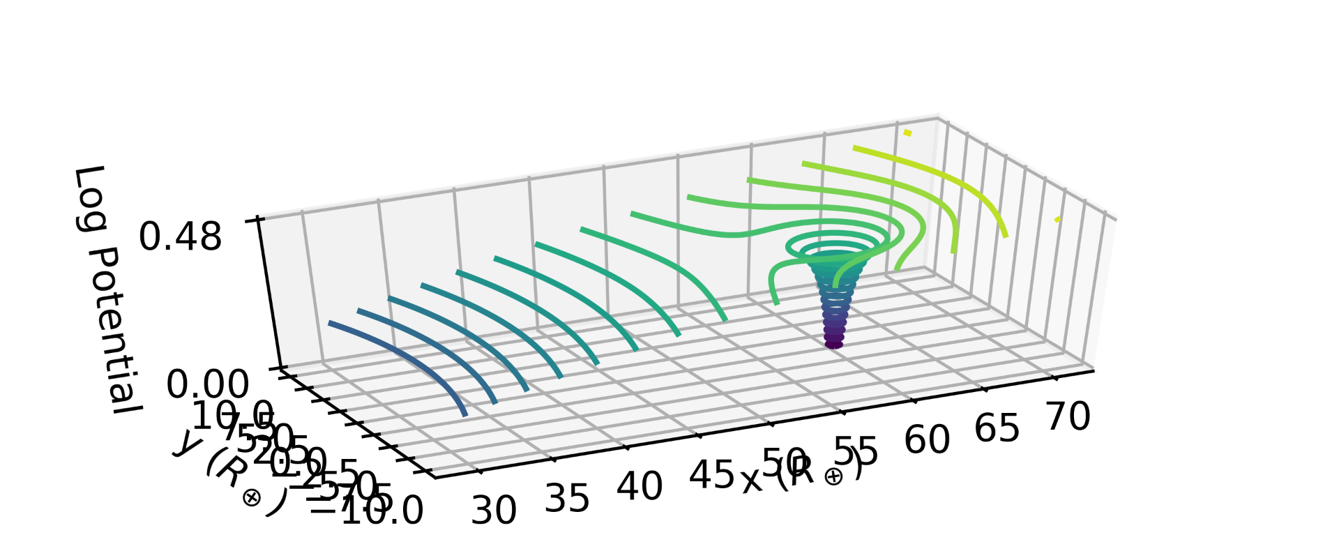
Now you can see that the “mountain pass” actually looks like a narrow gateway. This becomes clearer if you zoom in on the moon:

If you want to get up and over by using the least amount of energy (and thereby the least amount of fuel) then you would want to go right through the center, following the yellow V  up to where the color turns just a little green and then turns back (down) to yellow.  This shows that it’s a rather narrow mountain pass, so maybe it’s better to describe it as a gateway.

It is tempting to try to identify the “gateway” point as the Earth/Moon  Lagrangian Point L1, but it’s not, although they are probably close.   At the L1 Lagrangian point the Earth’s gravity is just slightly stronger than the Moon’s, such that an object there would orbit the Earth with the same orbital period as the moon (and thus if left there would simply follow along  with the moon, sort of like flying in formation).   The whole analysis presented here neglects the fact that the moon is actually in motion around the Earth, and to the extent that we are ignoring that motion the mountain pass is essentially the L1 Lagrange point.  To really get it right we would want to add the “effective” potential for an orbiting object.

Visualized with  Contour Lines

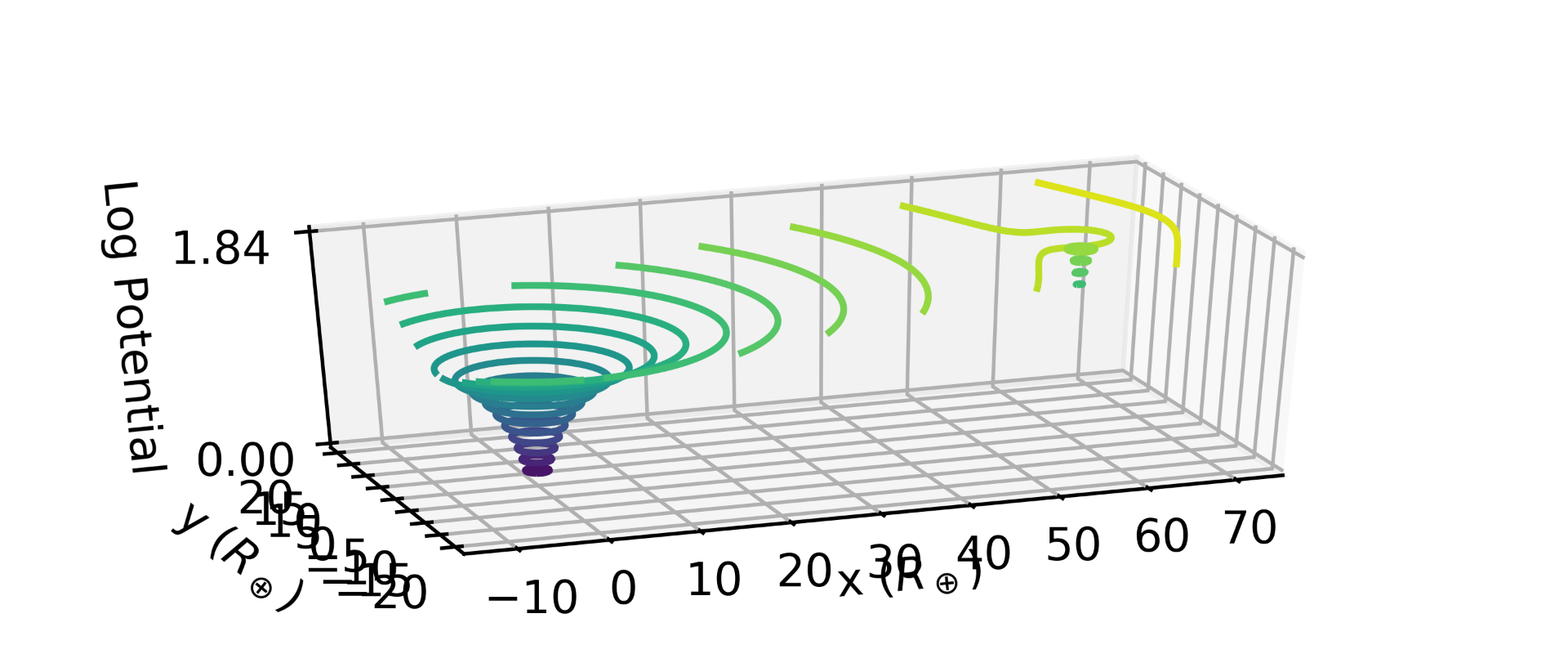
One friend I showed this all to had a little trouble visualizing the idea with the false color map, because the colors can look like “bumps”.   So I also plotted the surface using just contour lines, with the following result:

I like how one of the contour lines, which starts out “downhill” from the moon, actually loops back behind the moon.   This representation is the closest to a topographic (“topo”) map, where contour lines show elevation (and thus also gravitational potential energy).

That figure just shows the moon, but when you back out a bit to show both the Earth and Moon it also helps cement the idea of  gravitational potential as elevation:

Derivation of the Gravitational Potential

For completeness, here is my derivation of the expressions used in the script for the gravitational potential.  To start, the gravitational potential (symbol V) is the gravitational potential energy (symbol U)  divided by the mass of the spacecraft.  Dividing by the mass of the spacecraft makes the result proportional to U but independent of m, and thus we can think of it as being a property of the space at that point, independent of what is there.   And to get the potential energy, just as with electricity, multiply the potential by the amount of “charge” (in this case mass) at that position: U=Vm.   Now we just need to compute V.

To get the gravitational potential energy we can start with the force between the Earth or Moon and the spacecraft, which is given by Newton’s Law of Gravitation:

where M is the mass of the planetary body, m is the mass of the space ship, d is the distance between the two (center to center) and G_N is Newton’s constant of gravitation.  This is the magnitude of the force — the direction is of course attractive, through the centers of mass of both bodies.   If we integrate this, from the surface of the Earth up to the position of the space ship, we get the gravitational potential energy. Then, to get the potential we divide by the mass m of the spacecraft to get
This equation holds for both the Earth and the Moon (for different values of M), and we can simply add the two to get the total gravitational potential at any position.

The code I used to make the images is available as a github gist.

Notes