CosmicWatch Project, Episode 1: Getting Started

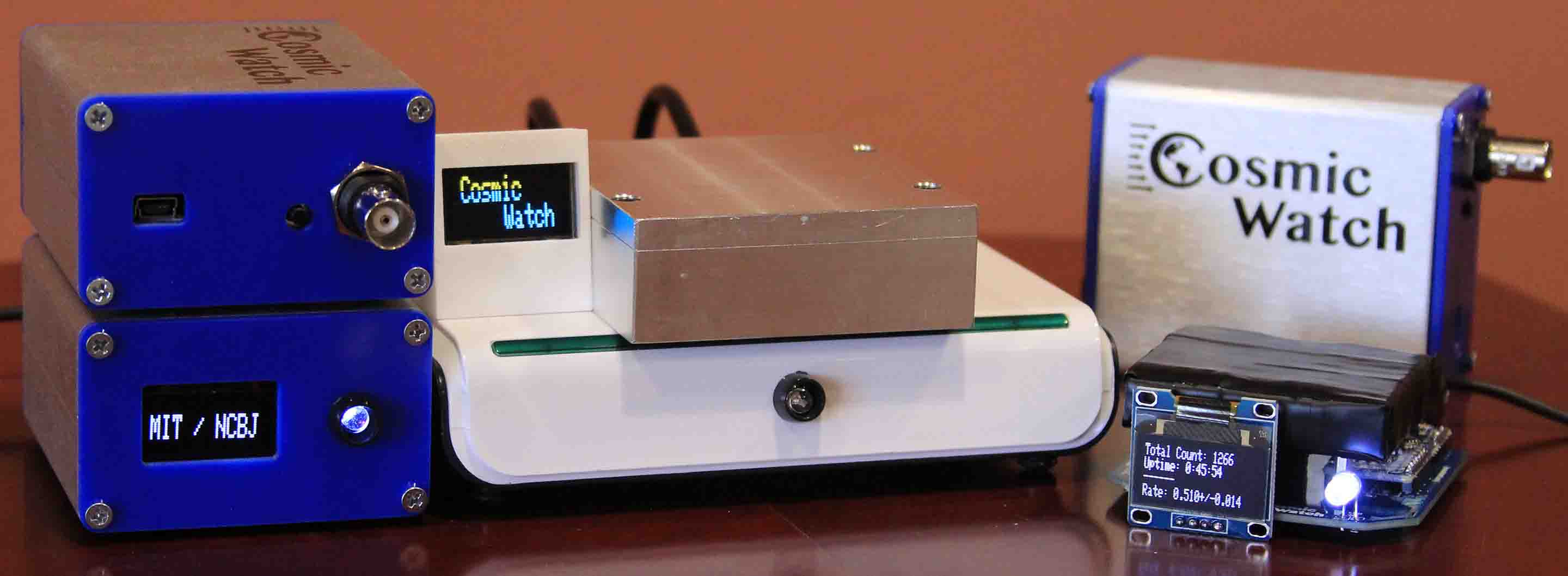
CosmicWatch is an inexpensive “home-built” cosmic ray detector designed by physicists at the Laboratory for Nuclear Science at MIT.   You can read more about it here: http://cosmicwatch.lns.mit.edu/about

The claim is that a college student can build one of these as a project for about $100 in about 4 hours1.    I’m skeptical, but it’s an interesting idea, so I’m going to put it to the test and build one myself.   I’m no longer a college student, but since I teach them, I want to see if this would be a viable project for our students, or even for local high school students.

I’ve been interested in cosmic rays for some time.   As an undergraduate I spent a summer working for the University of Utah helping to construct a large cosmic ray detector called the Fly’s Eye2 out in the desert near Dugway, UT.   As a graduate student at Yale I performed a simple coincidence experiment to detect cosmic rays, up in the attic of the physics building.   As an Assistant Professor at Vassar College my Modern Physics Laboratory course included an experiment to measure the lifetime of muons from cosmic rays3.   (I didn’t design it, but I did add some computer automation to the data acquisition.)

More recently, I collaborated with a group from the Education office at Fermi National Accelerator Laboratory (Fermilab) to create an “e-Lab” for high school students using data from the LIGO experiment4.   That’s not about cosmic rays, but that e-Lab was modeled on a cosmic ray e-Lab5  they created for their QuarkNet6 project.    By 2007 or so they had made several important advances in developing cosmic ray detectors that could be used by high school students.   They created a PCI card for data acquisition which could be put in just about any school PC, and they had found a way to isolate the high voltages normally needed to drive a Photomultiplier Tube (PMT).    The whole cost for a school to get started and join the detector network was, roughly, only around $2000.    So now, a bit over ten years later, here is a comparable detector for (they claim) only $100.    I have to check this out.

Instead of one long story, this will be a series of brief postings as the projects progresses.    The post you just read introduced the idea, so it corresponds to the first part of the CosmicWatch “How to build it?” page.   The next thing to look at is Purchasing Components.

References

  1. “CosmicWatch – How to Build it”  http://cosmicwatch.lns.mit.edu/detector#steps
  2. “A ‘New’ Experiment (1981)”, by the Telescope Array Project, http://www.telescopearray.org/index.php/history/the-fly-s-eye-1981-1993
  3. “Measuring the Lifetime of the Cosmic Ray Muon”, Vassar College Modern Physics Laboratory, v. 1.03 of 29 January 2003.
  4. “LIGO e-Lab”, https://www.i2u2.org/elab/ligo/home/project.jsp
  5. “Cosmic Ray eLab”, by the I2U2 collaboration,  https://www.i2u2.org/elab/cosmic/home/project.jsp
  6. QuarkNet, https://quarknet.org/

Raspberry Pi Initial Configuration

Whenever I flash a new SD card with a Raspbian image, there are a number of configuration steps that are needed to tune the configuration.    This post is just to record the steps for my own future reference. It’s based on the latest (as of this writing) release,  which is Raspbian Stretch.

    1. Edit the file /boot/config.txt to set (or uncomment) the following:
      hdmi_safe=1
      hdmi_force_hotplug=1
      You can also adjust the pixel overscan settings for your monitor, if needed, and increase config_hdmi_boost if that helps. But those are the most important two (for me, at least).
    2. Run the configuration utility
      $ sudo raspi-config
      and make the following adjustments:

      • 2 Network Options:
        • N1 Hostname:set it to something useful and specific to the project
        • N2 wifi:  if you are connecting to the Internet via wifi, enter the SSID and password here.
        • N3 Predictable Network Interface Names: DISABLE this (set it to NO) so that you get back simple interface names like “eth0” and “wlan0”.   More details about this may be found at https://www.freedesktop.org/wiki/Software/systemd/PredictableNetworkInterfaceNames/
      • 3 Boot Options:
        • B1 Desktop/CLI: usually set this to Command Line Interface (CLI)
        • B3 Splash Screen: turn this off, so you can see the boot process
      • 4 Localization Options:
        • I1 Change Local: change it to en_US
        • I2 Timezone: change to your local timezone (eg. America/New York)
        • I3 Keyboard: Select Generic 105-key PC and English (US). You can also set special keys here.
      • 5 Interface Options:
        • P2 SSH: enable it, so you can ssh into the pi and work on it even when it’s headless.
        • P5 Serial: disable this, unless you actually have a serial port device to connect to it.
        • P1 Camera: enable this if you intend to use the Raspberry Pi camera.
      • 6 Advanced Options:
        • A1 Expand Filesystem: expand the filesystem to use the entire SD card. (this might now be done automatically at first boot).
    3. Install emacs (so I can edit things easily, though nano is not bad):
      $ sudo apt-get install emacs
      I also like tcsh, so I’ll install that now too.
    4. Update and Upgrade:
      $ sudo apt-get update
      (Remember, this just updates the package database, which “resynchronize the package index files from their sources”1)
      $ sudo apt-get upgrade

(This actually installs the newest versions of all the packages, at least for the Debian version you are using. It does not upgrade to a newer version of Debian.)

  1. Set new passwords:
    $ sudo passwd root    to set a new root password
    $ passwd                  to set a new password for user “pi”

References

  1. apt-get man page

Van de Graaaaafffff!

My colleague and friend Glenn Geher from the New Paltz Psychology department was visiting our new building, and so I showed him around our teaching lab space.    He was especially excited about the Van de Graaff generator, so I gave him a little demo:


What’s happening? As I explained at the beginning, the device uses an electric motor to drive a rubber belt which carries electric charges (electrons) off of the metal sphere, leaving behind a net positive electric charge.   Here’s a good diagram from Wikipedia:

Figure 1: Schematic image showing the operation of a Van de Graaff generator.

Eventually, the electric charge on the sphere becomes so great that the electric field it creates is strong enough to break through the nearby air (which is called “di-electric break-down”) and a spark of charge jumps from the small electrode to the sphere.  This is a lot like what happens when a bolt of lightning jumps from the ground to a cloud, or vice-versa.  That’s the clicking sound you hear, even if you can’t see every spark.

Then I put the metal pie plates on top of the metal sphere.   The electric charge now builds up on the pie plates as well.   It’s a fundamental property of electric charges that like charges repel, while opposites attract.   Each pie plate is then, in turn, repelled by the metal sphere and the plates below it, and goes sailing up into the air.

In the video I say that the belt carries electric charges up and onto the sphere, which sounds backwards from what I described above.   But it’s really the same thing.   The belt actually takes electrons from the metal sphere, and electrons have negative electric charge, so this leaves behind extra positive electric charge.   You can just as well imagine that the belt brings extra positive charges up to the metal sphere;  the effect is the same either way.   In fact, being able to tell which kind of charge is actually moving  is a bit of a challenge.   Benjamin Franklin originally came up with the names “positive” and “negative” charge, based on his own idea of which kind was flowing where, and as it turns out he got it backwards.


Vernal Equinox in Wooster Hall: Irregular Interval Time-Lapse Animation

Vernal Equinox in Wooster Hall: Irregular Interval Time-Lapse Animation

Wooster Hall on the SUNY New Paltz campus was completely remodeled recently, and a neat new feature is an alignment of the skylight over the main stairway such that the bottom of the stairs is lit up at exactly solar noon on the Equinox  (both spring and fall).

This spring when I observed this I was inspired, on the fly, to create a time-lapse video of the event, using just my hand-held phone.   You can see the video here.

Making the time-lapse video from the still images was a fun little exercise in Python programming, and the purpose of this post is to show how I did it.   I need to start out by saying that this is all really crude compared to what one can do now with time-lapse photography, but it was what I was able to do with little background or training, so I wanted to at least record what I learned.

One of the challenges to deal with is that the images were not captured at regular intervals, since I was taking them by hand with my phone.   I tried to space them out about every minute, but sometimes it took longer (like when someone was in the way) and sometimes I took them more frequently (as we got closer to solar noon).   Even so, I wanted to make the video flow as smoothly as possible by adjusting the time between frames accordingly.    That lead me to choose to make an animated GIF instead of some other format, because an Animated GIF can have different time delays for different images, whereas most video has a uniform spacing between frames.

My previous experience making an animated GIF was using the command line convert tool from Image Magick, but even that assumes a standard frame rate and does not make it easy to change the delays individually for different frames.   Still, I knew that the time of each image was recorded in the JPG file, so in principle I could use that to adjust the time between frames, if I read that information programatically.   That lead me to choose to write a Python script to do the job.   And then looking at what was available in Python, I chose to use PIL, the Python Image Library.

The way it works, overall, is that you read in all the images into a list, then save the first image as a GIF, and at the same time tell it to append all the other images, with an array of different time durations to show each image.   For animated GIFs the time to show each frame is in hundredths of a second, so I simply scale down the time interval between when the pictures were taken to an appropriate amount in hundredths of a second.

I also needed to do some processing for each image, before it was added to the animation.
Because I held the phone horizontally (landscape) but the JPG files default to “up” being portrait mode, I had to rotate each image by 90 degrees.   I also wanted to scale down the size of the image to make a smaller animated GIF appropriate for a web page, rather than a full sized video.

To get started I imported PIL and set up some empty arrays to hold the images, the durations (time between frames), and the names of the original image files.

from PIL import Image

images = []
durations = []
prev_time = datetime.now()

The current time is saved in prev_time to start the process of computing the time between successive photos. At this point I just needed a value which is both a ‘dateime’ object and somehow signals that it’s not a part of the sequence of times, which this does by being so much later than the first image.

Before reading in images, I needed an ordered list of the file names.  The file names are simply IMG_2921.JPG up to IMG_2821.JPG, in order.   I used the os module and made sure that the list was properly sorted:

import os

# Get a list of .JPG files
filenames = []

for file in os.listdir('.'):
    name, ext = os.path.splitext(file)
    # Only files, only .JPG files
    if os.path.isfile(file) and ext == ".JPG":
        filenames.append(file)
print "Found ", len(N), "image files.  "

filenames.sort()

With this list I was able to use PIL to read in each image file, rotate the image, resize the image, and then save the image in a list:

for file in filenames:
    img =  Image.open(file)
    rotimg = img.rotate(-90,expand=1)
    newsize = ( int(rotimg.size[0]/scale), int(rotimg.size[1]/scale) )
    frame = rotimg.resize(newsize)
    images.append(frame)

I set scale to 5.0 to reduce the size to 1/5 the original.

After saving each frame in the animation, I get the timestamp from the EXIF data in the original image, which just happens to be element 36867 of the EXIF property array. (You can look this up — I certainly had to). From this I computed the time duration for each frame, in hundredths of a second:

    # Duration of frame comes from actual time difference between photos

    exif = img._getexif()         # JPEG photo metadata (EXIF)
    datestamp = exif[36867]       # date/time the photo was taken
    img_time = datetime.strptime(datestamp,"%Y:%m:%d %H:%M:%S") # parse datestamp
    deltat = img_time - prev_time # difference as "timedelta" objects
    dt = deltat.total_seconds()   # difference in seconds (or fraction of)
    if dt < 0:                    # ignore the first one, it's bogus
        durations.append(dt*100.0/speedup) # GIF duration is in 100ths of second
    prev_time = img_time          # Save timestamp for next iteration

In Python, differences between ‘datetime’ objects are ‘timedelta’ objects1 and then we convert that to a float value in seconds, called dt, and rescale that to hundredths of a second. The scale factor speedup was set to a value of 30.0 to get a reasonable speed for the animation.

Notice that the duration of the frame is not saved for the first frame. That means that for the 99 images in the collection, there are only 98 durations (and of course they are all different). This turns out to be almost what is needed for the next step, putting all the frames together into the animation.

After this loop over all frames, the rotated and scaled images are in the list named images, the duration for each frame is in the list durations, and it’s time to put them all together. The way this is done is to write one frame image, and then tell PIL to append to it the list of the other images, with the list of durations.

print "Writing the movie..."
first = images.pop(0)
durations.append(100)     # pause 1 second at end of loop
print len(images), len(durations)
first.save("WoosterMovie.gif",save_all=True,
                              append_images=images,duration=durations,loop=47)

With 99 images in the list, the first is put into the variable first (and removed from the images list, which now has 98 elements. Meanwhile, I had to add another element to the end of the durations list, so now there are 99 durations. That makes some sense, because there are 99 images overall, but the mis-match between the length of the images list and the durations list was very confusing to me, and is probably the most important reason for writing this posting. Which is why I even printed the lengths to verify them when I finally got it figured out. But as you can see from the comment, it also means I could control the length of the pause at the end of the animation before it repeated. Also as you can see, you “save” the first image, and then pass the other images and durations as parameters, which seemed kinda weird at first, but that’s how the API works, so that’s how you do it. Hopefully this working example is useful to someone else, or at least to me in the future when I forget all this.

References
  1. Python Documentation, 8.1.4. datetime Objects https://docs.python.org/2/library/datetime.html#datetime-objects

Vernal Equinox in Wooster Hall

Vernal Equinox in Wooster Hall

The newly updated Wooster Hall has a neat feature at the bottom of the staircase between the first and second floors.  Above that stair  there is a large skylight with 4 windows, and at the bottom of the stairs there are markings on the floor that show where the shadows between those windows will be at solar noon on the Vernal Equinox (see the image above).

I was able to observe this phenomenon in some detail on Tuesday, 19 March 2018 (which was actually the day before the equinox, but the weather was expected to be cloudy the next day, and indeed it was). When I arrived I found a nice corner to observe from, and although I had not planned to do so ahead of time, I ended up taking a picture just about every minute (and more frequently right around solar noon) for an hour or so. After a little research I was able to write a Python script to put the images together in the following animated GIF  (keep your eyes on the shafts of sunlight moving across the floor):

The speed  is a little rough — I was aiming for one second of animation for one minute of real time but apparently I still need to make some adjustments, and even then it might depend on which browser you are using.

It was a little tricky to do this right, because I was not able to take the photos at regular intervals, and so the duration of each frame in the animation had to be computed from the time of the photo, which was extracted from the EXIF metadata. In case it is of some interest, the details of how I created this animations are in my next post: “Vernal Equinox in Wooster Hall: Irregular Interval Time-Lapse Animation

Repairing a Cenco 33031 Power Supply

Figure 1: Cenco 33031 Low Voltage Power Supply

by Laurence Rowe and Eric Myers

We use the Cenco 33031 Low Voltage Power Supply (Figure 1) for several of our electricity and magnetism labs.   It can provide variable DC up to 6 Volts at up to  5 Amps, and it can provide a steady AC voltage at around 22 VAC.

Unfortunately, our students sometimes exceed the 5 Amp DC limit and damage the supply, rendering it useless.   The problem is almost always the main power transistor.   We have even tried adding a 5A fuse in the DC output circuit, but the power transistor blows out much more quickly than a fuse.  We recently switched some devices to use 4A fuses, with some success, but in the case of a short circuit this small difference will probably not matter; the power transistor will blow first.

Presented below are step-by-step instructions for replacing the power transistor.  Another component that might need to be replaced is an LM317 voltage regulator.   We will add instructions for replacing that sometime in the future.   Meanwhile, when the DC fails, the first thing to try is replacing the power transistor.

Preparations

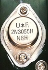
Figure 2: 2N3055 Power Transitor
Figure 2: 2N3055 

Before you get started, you will need the replacement part(s) and some tools:

  • Phillips screw driver
  • Soldering iron
  • 2N3055 power transistor (Figure 2)
  • Thermal paste
  • Replacement mica heat shield for the 2N3055
  • LM317T voltage regulator (optional)

You may be able to re-use the mica heat shield, but you won’t know that for sure until you remove the power transistor, so you’ll want to have one on-hand just in case.

While it is also optional, it can be helpful to use a plastic compartment box  to hold the screws and other parts during disassembly.    If you don’t have a plastic box, an egg carton works just as well.

See the addendum below for an estimate of the time required for the repair.

 Replacing the Power Transistor

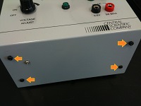
  1. Remove the 8 small case screws (see Figure3), gently lift the cover, and slide it to the right.

    Figure 3: Case screws.
    Figure 3: Case screws.
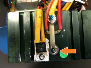
  2. Remove the 2 screws holding the heat sink to the bottom of the case (shown in Figure 4).  Be careful not to bend or break the leads on the voltage regulator, which is the black chip with 3 leads which is attached to the heat sink.   Those leads can break off easily.

    Figure 4: Heat sink screws.
    Figure 4: Heat sink screws.
  3. You will find two components connected to the heat sink.   The power transistor sits on one side of the heat sink and is connected to it by screws at both ends.    On the other side of the heat sink is an LM317T voltage regulator, a smaller black chip with 3 leads. There are tie wraps around bundles of wires for neatness. Remove these as needed (and replace on reassembly if you can).Start with the screw at the far “plain” end of the transistor – the one without a wire attached (see Figure 5).  Remove and save the nut, washer, lock washer, and the screw.

    Figure 5: "Plain" transistor screw - no wire.
    Figure 5: First transistor screw.
  4. Then go to the other end of the transistor, and remove the top nut, washer, lock washer, and the wire lug.  You can’t see the color of the wire in the picture because of the yellow insulating sleeve, but you’ll easily see that this is the white wire.  There is another nut and washer underneath the first.
  5. Heat the solder and remove the red and orange wires from the power transistor, shown in Figure 6.  Take care to avoid excess heat or you will damage the plastic insulator between the two wires.
    Figure 6. Red and Orange wires connecting to Power Transistor.

    Note the placement of the wires.   The thicker red wire is farthest from the voltage regulator (black chip) and the slightly thinner orange wire is closer to the voltage regulator.

  6. Now remove the remaining nut, washer and screw from the power transistor and save these.
  7. Once the wires have been removed, you can clip the leads on the power transistor as close to the heat sink as possible to facilitate removal.
  8. Pull up on the plastic insulator by the center tab (the part which was between the red and orange wires).  Push the cut leads from the back to release the transistor.
  9. You can leave the mica insulator in place if it is still contacting the heats sink.  If it comes off the heat sink then you’ll need to gently clean the surface and either reuse it (if intact) or replace it.   Be careful, the mica breaks easily.
  10. In any case, spread a fresh layer of heat compound over the mica insulator to make a good thermal connection to the new power transistor.
  11. Place the new power transistor where the old one was, with the leads through the holes in the heat sink and through the holes in the plastic insulator.   It may not be obvious at first, but there is a slight asymmetry — the leads are offset from the centerline — so that you can only put the transistor in one way, and only orient the plastic insulator one way.
  12. Reinstall the screws at both ends of the power transistors.   Keep in mind that the longer screw goes on the end that will connect to the wire lug on the white wire.   It’s easiest to connect the wire lug last, when the other screws are holding the power transistor in place.
  13. Re-solder the orange and red wires to the power transistor.   As shown in Figure 6, the orange wire is closest to the voltage regulator (black chip) and the red wire is farthest from it.
  14. Test the repair before you screw the heat sink back in place or the cover.  The power supply should now go up to at least 6VDC when turned all the way up.   If not, you’ll have to check your work more carefully.   You may have to replace the voltage regulator too.
  15. Reattach the heat sink to the case.
  16. Close the case with the 8 case screws.

The last thing we will mention is that some students have taken to turning the power supply on it’s side, so that the “top” faces forward instead of upward.   The case screws can then scratch the table, so I’ve been adding rubber feet next to the case screws to prevent such scratches.

Addendum

12 March 2019:   The last time I made this repair it took me 35 minutes from cracking the case open to closing it up (all 8 screws), and I had done it before, but not recently.   If I was to do another immediately I could probably get the time under half an hour, but if you’ve never done this before then plan to spend at least twice as long.


Skip to toolbar